Building an Analytics Cube in Microsoft Fabric
In today’s data-driven world, the ability to analyze and interpret vast amounts of information is crucial for making informed business decisions. Whether you’re a financial analyst seeking to uncover trends in revenue and expenses, or a sales manager aiming to optimize your team’s performance, having the right tools at your disposal can make all the difference. This is where analytics cubes come into play.
An analytics cube is a multi-dimensional database that allows users to slice and dice data across various dimensions, providing a powerful way to explore and visualize complex datasets. Accessible through familiar tools like Excel, Power BI, ADS, SSMS or an end-point in Service, analytics cubes cater to users of all skill levels, from novice spreadsheet (no-code) users to seasoned data scientists.
In this post, I’m going to walk through the basic steps to create an analytics cube in Microsoft Fabric from data ingestion to final product.
1. Designing the Structure
For the structure, I decided to go with the trusty medallion (or curated) architecture. That is, an ‘ingestion’ store of raw data, a store of transformed data, and a final modelling store with the final, curated and consolidated data, measures and relationships built in.
At it’s most simple, it might look like the above. With steps to bring data into a Lakehouse/DWH, steps to transform that data and deposit it in a silver/transformed layer, then more steps to consolidate that data in a final store, before downstream reporting/reports are built on top.
By the time I finished, my workflow looks like:
2. Data Ingestion
So the first step is to create a new Lakehouse (store). If you’ve used the process flow in the Fabric workspace, it’s easier to select the ‘Bronze Data’ flow -> Add item -> Lakehouse. My convention is to always name Lakehouses beginning with LH. e.g., LH_Bronze, LH_Project_Ingestion, etc.,
With our Lakehouse set up and ready to go. We need to populate it with raw data. The ingestion method you use to populate this depends on your or your company’s tech stack and where the primary data sits. Often times, data sits across multiple platforms so your ingestion techniques might need to adapt to this. You could use:
- Pipelines with ‘Copy Data’ activity (I personally used this when my data storage was in GCP)
- Pipelines with Shortcuts
- Dataflow Gen2
- Notebooks
- Eventstreams (RTD)
- Manually upload CSV/JSON/Parquet to LH and load to Delta Tables
3. Transform
Now you have your raw data (system generated transactions, for example), it’s time to transform it. Perhaps you have different streams from different sources that you’ll need to consolidate. This is the step to ensure schemas are standardized. So if one source table contains a column called “Product_CD” and another table is called “Prod_code”, you need to ensure these both share the same name. Transformations can be done in PySpark notebooks or Dataflows.
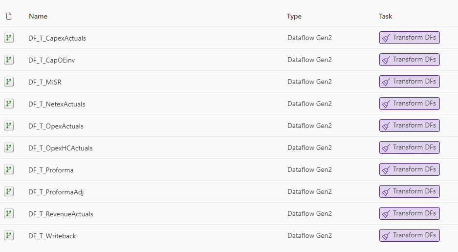
When I was building a Financial cube, I created separate dataflows for each stream (Revenue, Operational Expenses, Cost of Sales, Capital Expenditure, Incremental Service Revenue, Writeback);

In these dataflows, I set the storage destination to my curated (silver) Lakehouse. I standardized the schemas, performed any necessary merges to static files (e.g., FX rates). I could also create additional tables to append manual journal entries or corrections without saving that table to a destination.
4. Consolidate
With my data now all in the format I want it to be, stored in separate tables (for faster processing and redundancy in case of source failure), I can begin consolidation. I used a PySpark notebook for this instead of a Dataflow gen2 as Spark is significantly better at processing large volumes of data. I needed to process 25m rows regularly, so a DF Gen2 which was taking ~25 minutes per refresh just wasn’t going to cut it.
from pyspark.sql import SparkSession
from pyspark.sql.functions import lit

# Define the columns to select
selected_columns = ["GL_PERIOD_START_DT", "CUST_NBR", "GL_COMPANY_CD", "GL_BUSINESS_AREA_CD", "GL_PROFIT_CTR_CD",
                    "GL_PROFIT_CTR_REGION_CD", "GL_LOB_CD", "GL_MGMT_PRODUCT_CD", "GL_ACCOUNT_CD", "ENTERED_CURRENCY_CD",
                    "ACCOUNTED_CURRENCY_CD", "ENTERED_AMT", "ACCOUNTED_AMT", "USD_AMT", "USD_BUDGET_AMT", "CUST_NAME",
                    "ULTIMATE_CUST_NBR", "ULTIMATE_CUST_NAME", "SAP_BPC_GL_ACCOUNT_ID", "LOCAL_EURO", "D_ACCOUNTED_AMT_EURO",
                    "TABLE", "SCENARIO", "LocalToEUR", "GL_REGION_CD", "GL_CUST_TYPE_CD", "GL_COST_CENTER_CD", "DELETION_IND",
                    "PA_PROJECT_NBR", "PROJECT_APPROVAL_CD", "Program_CD", "HC_TYPE"]

# Function to select columns and add missing columns with null values - do not modify this code
def select_and_add_missing_columns(df, columns):
    for col in columns:
        if col not in df.columns:
            df = df.withColumn(col, lit(None))
    return df.select(*columns)


# Read and process tables. If other tables need to be consolidated into the data table, add them here
df1 = select_and_add_missing_columns(spark.read.format("delta").load("Tables/ProformaTransformation"), selected_columns)
df2 = select_and_add_missing_columns(spark.read.format("delta").load("Tables/Capex_Actuals"), selected_columns)
df3 = select_and_add_missing_columns(spark.read.format("delta").load("Tables/Netex_Actuals"), selected_columns)
df4 = select_and_add_missing_columns(spark.read.format("delta").load("Tables/Opex_Actuals"), selected_columns)
df5 = select_and_add_missing_columns(spark.read.format("delta").load("Tables/Opex_HC_Actuals"), selected_columns)
df6 = select_and_add_missing_columns(spark.read.format("delta").load("Tables/Revenue_Actuals"), selected_columns)
df7 = select_and_add_missing_columns(spark.read.format("delta").load("Tables/MISR_All"), selected_columns)
df8 = select_and_add_missing_columns(spark.read.format("delta").load("Tables/Capex_CapOE_Inv_Actuals"), selected_columns)
df9 = select_and_add_missing_columns(spark.read.format("delta").load("Tables/ProformaAdj"), selected_columns)

# Combine loaded dataframes, allows for missing columns
combined_df = df1.unionByName(df2, allowMissingColumns=True) \
                 .unionByName(df3, allowMissingColumns=True) \
                 .unionByName(df4, allowMissingColumns=True) \
                 .unionByName(df5, allowMissingColumns=True) \
                 .unionByName(df6, allowMissingColumns=True) \
                 .unionByName(df7, allowMissingColumns=True) \
                 .unionByName(df8, allowMissingColumns=True) \
                 .unionByName(df9, allowMissingColumns=True)

# Write the consolidated table to LH_NFC_Modeling/Tables/Data
combined_df.write.format("delta").mode("overwrite").save("abfss:/.../Tables/Data")
5. Model and Measures
With the data now in my final Lakehouse, it’s time to build the relationships, which can be done using the default semantic model (or by creating new semantic models for specific purposes).
With the relationships built, I can move on to making measures. I created a table called “DimMeasures” using my dimension dataflow, as it’s worth noting that if a table gets dropped from the Lakehouse (e.g., if you break something or configure it incorrectly) you will lose all the measures assigned to that table.
Some examples of measures in a Financial Analysis Cube would be calculation of monthly actuals, budgets & forecasts, period analysis, etc.,
Actual @ EUR Budget =
VAR Current_AC_Level_3 = SELECTEDVALUE ( DimAccount[AC_Level_3] )
VAR Result =
    SWITCH (
        TRUE (),
        Current_AC_Level_3 IN { "Revenue", "Cost of Sales" }, CALCULATE (
            SUM ( Data[D_ACCOUNTED_AMT_EURO] ),
            DimLOB[Tier1_Desc] = "Exclude Internal"
        ),
        Current_AC_Level_3 = "Run Rate", SUM ( Data[D_ACCOUNTED_AMT_EURO] ),
        SUM ( Data[D_ACCOUNTED_AMT_EURO] )
    )
RETURN
    Result


Forecast @ EUR Budget =
CALCULATE(
SUMX(
    Writeback,
    Writeback[LOCAL_AMT] * Writeback[LocalToEUR]
), Writeback[SCENARIO] = "Forecast")


MvF EUR = [Actual @ EUR Budget] - [Forecast @ EUR Budget]
6. Access, Release and Next Steps
With the cube now being fully set up, all that’s left to do is to assign users or distribution lists access to the Lakehouse. Without access to the workspace, providing ReadAll and Build access will let users access the model and measures through the following ways:
- SQL Analytics EndPoint in Service
- Power BI (connecting to the default semantic model)
- Microsoft Excel (via Get Data -> Power Platform -> Power BI Datasets)
- Azure Data Studio / SQL Server Management Studio via the SQL Analytics Endpoint
Users will not be able to create views or measures, nor will they be able to modify relationships, run PySpark notebooks or in any way ‘break’ the model. From here, the curated model can serve as the single source of truth for any downstream reporting or analyses, and, using custom semantic models, or RBAC/One Security, OLS/RLS, you can customize who can access what and with which tools.

Leave a Reply